Abstract
Infinite impulse response filters are an essential building block of many time-varying audio systems, such as audio effects and synthesisers. However, their recursive structure impedes end-to-end training of these systems using automatic differentiation. Although non-recursive filter approximations like frequency sampling and frame-based processing have been proposed and widely used in previous works, they are approximations and cannot accurately reflect the gradient of the original system. We alleviate this difficulty by re-expressing a time-varying all-pole filter to backpropagate the gradients through itself, so the filter implementation is not bound to the technical limitations of automatic differentiation frameworks. This implementation can be employed within any audio system containing filters with poles for efficient gradient evaluation. We demonstrate its training efficiency and expressive capabilities for modelling real-world dynamic audio systems on a phaser, time-varying subtractive synthesiser, and feed-forward compressor. We make our code available and provide the trained audio effect and synth models in a VST plugin.

Figure 1: The forward (left) and backpropagation (right) flow chart of a third-order time-varying all-pole filter.
Listening Samples
We provide listening examples for our experiments modeling a phaser (Electro-Harmonix Small Stone), a time-varying subtractive synthesizer (Roland TB-303 Bass Line), and a feedforward-compressor (LA-2A Leveling Amplifier). All three systems are trained to model some target analog audio in an end-to-end fashion using gradient descent.
1. Phaser (Electro-Harmonix Small Stone)

Figure 2: Discrete-time phaser model considered in this work, where K = 4. APF represents a time-varying all-pass filter with difference equation and BQ is a biquad filter.
For our first experiment, we use our time domain filter to model the Electro-Harmonix SmallStone phaser pedal using the differentiable phaser architecture shown in Figure 2. The Electro-Harmonix SmallStone's circuit consists of four cascaded analog all-pass filters, a through-path for the input signal, and a feedback path which means it is topologically similar to our phaser implementation. The pedal consists of one knob which controls the LFO rate, and a switch that engages the feedback loop.
| Parameter Config. |
LFO Rate | Feedback | Hop Size L / Fs |
Input | Target | TD (Ours) | FS |
|---|---|---|---|---|---|---|---|
| SS-A | ≈ 2.3 Hz | off | 10 ms | ||||
| SS-B | ≈ 0.6 Hz | off | 40 ms | ||||
| SS-C | ≈ 0.09 Hz | off | 160 ms | ||||
| SS-D | ≈ 1.4 Hz | on | 10 ms | ||||
| SS-E | ≈ 0.4 Hz | on | 40 ms | ||||
| SS-F | ≈ 0.06 Hz | on | 160 ms |
Table scrolls horizontally if space is limited.
2. Time-varying Subtractive Synthesizer (Roland TB-303 Bass Line)

Figure 3: Diagram of the differentiable synth modelling process. Our time-domain filter component is shown in green.
For our second experiment, we use our time domain filter to model the Roland TB-303 Bass Line synthesizer which defined the acid house electronic music movement of the late 1980s. The TB-303 is an ideal synth for our use case because its defining feature is a resonant low-pass filter where the cutoff frequency is modulated quickly using an envelope to create its signature squelchy, “liquid” sound. We model it using the time-varying subtractive synth architecture shown in Figure 3 which consists of three main components: a monophonic oscillator, a time-varying biquad filter, and a waveshaper for adding distortion to the output. The dataset is made from Sample Science’s royalty free Abstract 303 sample pack consisting of 100 synth loops at 120 BPM recorded dry from a hardware TB-303 clone.
Table 2.1: Entire test set concatenated together.
| Filter Config. |
Inference Method |
Target | TD (Ours) | FS 128 | FS 256 | FS 512 | FS 1024 | FS 2048 | FS 4096 | LSTM 64 |
|---|---|---|---|---|---|---|---|---|---|---|
| Coeff. | TD | N/A | ||||||||
| Coeff. | FS | N/A | N/A | |||||||
| Low-pass | TD | N/A | ||||||||
| Low-pass | FS | N/A | N/A | |||||||
| RNN | TD | N/A | N/A | N/A | N/A | N/A | N/A | N/A |
Table scrolls horizontally if space is limited.
Table 2.2: Five different test set audio clips repeated 16 times each for easier comparison.
| Example Number |
Filter Config. |
Inference Method |
Target | TD (Ours) | FS 128 | FS 256 | FS 512 | FS 1024 | FS 2048 | FS 4096 | LSTM 64 |
|---|---|---|---|---|---|---|---|---|---|---|---|
| 1 | Coeff. | TD | N/A | ||||||||
| 1 | Coeff. | FS | N/A | N/A | |||||||
| 1 | Low-pass | TD | N/A | ||||||||
| 1 | Low-pass | FS | N/A | N/A | |||||||
| 1 | RNN | TD | N/A | N/A | N/A | N/A | N/A | N/A | N/A | ||
| 2 | Coeff. | TD | N/A | ||||||||
| 2 | Coeff. | FS | N/A | N/A | |||||||
| 2 | Low-pass | TD | N/A | ||||||||
| 2 | Low-pass | FS | N/A | N/A | |||||||
| 2 | RNN | TD | N/A | N/A | N/A | N/A | N/A | N/A | N/A | ||
| 3 | Coeff. | TD | N/A | ||||||||
| 3 | Coeff. | FS | N/A | N/A | |||||||
| 3 | Low-pass | TD | N/A | ||||||||
| 3 | Low-pass | FS | N/A | N/A | |||||||
| 3 | RNN | TD | N/A | N/A | N/A | N/A | N/A | N/A | N/A | ||
| 4 | Coeff. | TD | N/A | ||||||||
| 4 | Coeff. | FS | N/A | N/A | |||||||
| 4 | Low-pass | TD | N/A | ||||||||
| 4 | Low-pass | FS | N/A | N/A | |||||||
| 4 | RNN | TD | N/A | N/A | N/A | N/A | N/A | N/A | N/A | ||
| 5 | Coeff. | TD | N/A | ||||||||
| 5 | Coeff. | FS | N/A | N/A | |||||||
| 5 | Low-pass | TD | N/A | ||||||||
| 5 | Low-pass | FS | N/A | N/A | |||||||
| 5 | RNN | TD | N/A | N/A | N/A | N/A | N/A | N/A | N/A |
Table scrolls horizontally if space is limited.
3. Feed-forward Compressor (LA-2A Leveling Amplifier)
For our third experiment, we use our time domain filter to learn the parameters for the Universal Audio LA-2A analog compressor. We optimise our proposed differentiable feed-forward compressor to match the target audio, examining its capability to replicate and infer the parameters of dynamic range controllers. We train and evaluate our compressor on the SignalTrain dataset, which consists of paired data recorded in 44.1 kHz from the LA-2A compressor with different peak reduction values.
| Config. | Peak Reduction |
Input | Target | TD (Ours) | FS |
|---|---|---|---|---|---|
| LA-D | 25 | ||||
| LA-E | 50 | ||||
| LA-F | 75 |
Table scrolls horizontally if space is limited.
Plugins
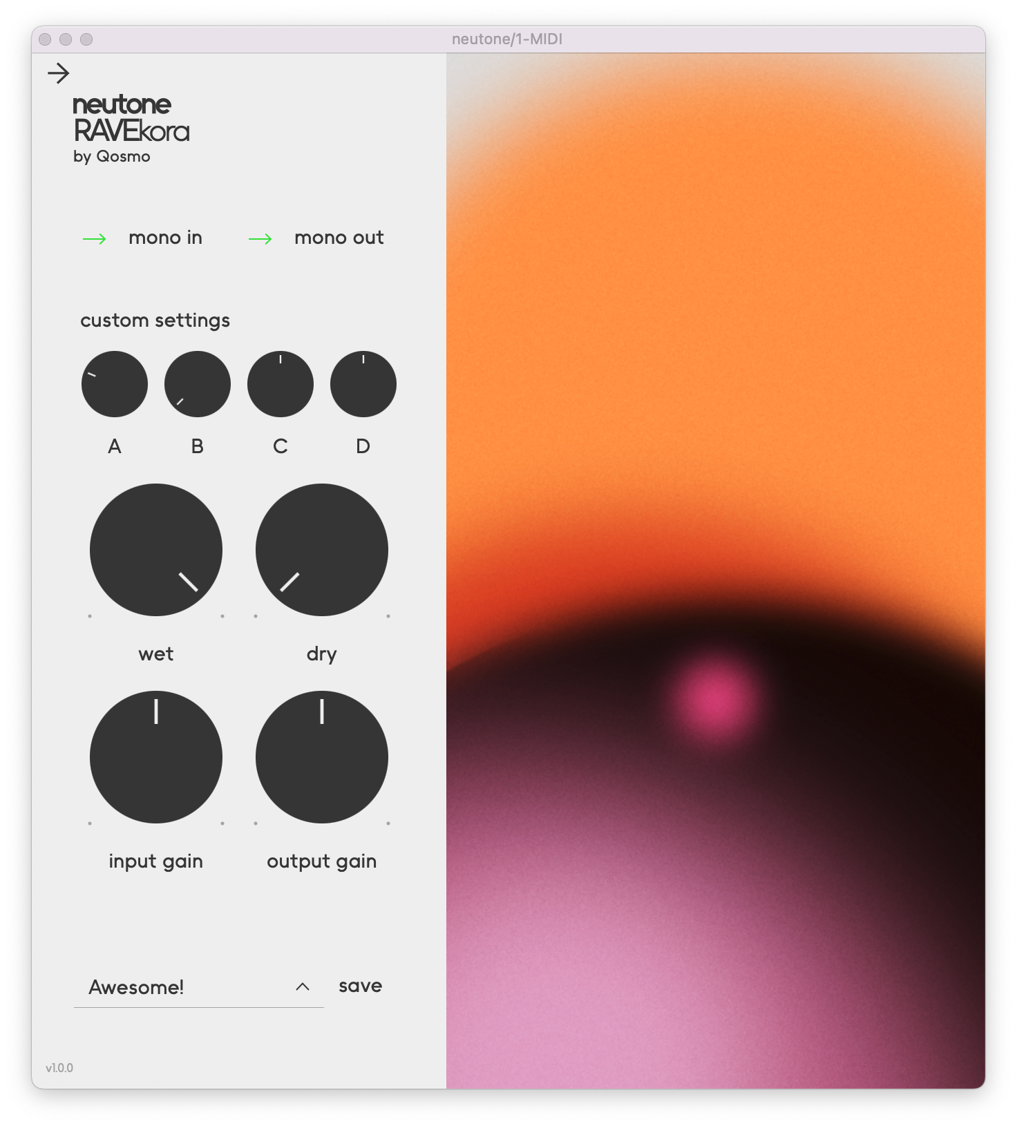
Figure 4: The Neutone FX plugin user interface.
We make the trained effect models accessible using the Neutone platform and SDK. This enables most users to experiment with the models via a real-time VST plugin in their preferred digital audio workstation (DAW) on arbitrary input audio. Older CPUs may struggle to run the models in real time.
Instructions
- Download and install the Neutone FX plugin.
- Download a model file from the links below.
- Open the plugin in your preferred digital audio workstation.
- Click on "load your own" at the top of the Neutone FX plugin interface and select one of the models you just downloaded.
- Use the four custom knobs to control the model.
Phaser
We provide the trained phaser model files for the six different parameter configurations explored in the paper. The phaser is controlled as follows:
- Knob A: LFO rate (0.05 Hz to 3 Hz)
- Knob B: LFO stereo offset (0 to 2π)
Phaser Neutone Files
- SS-A TD (feedback off, rate knob 3 o’clock (f0 ≈ 2.3 Hz))
- SS-B TD (feedback off, rate knob 12 o’clock (f0 ≈ 0.6 Hz))
- SS-C TD (feedback off, rate knob 9 o’clock (f0 ≈ 0.09 Hz))
- SS-D TD (feedback on, rate knob 3 o’clock (f0 ≈ 1.4 Hz))
- SS-E TD (feedback on, rate knob 12 o’clock (f0 ≈ 0.4 Hz))
- SS-F TD (feedback on, rate knob 9 o’clock (f0 ≈ 0.06 Hz))
Time-varying Subtractive Synthesizer
We first provide a time domain and frequency sampling version of the low-pass biquad configuration of our synth implementation without the modulation extraction neural network so that users can familiarize themselves with the synth and test whether it can run in real time on their CPU. The synth is controlled as follows:
- Knob A: Oscillator pitch (F#1 to C4)
- Knob B: Decaying envelope exponent (0.2 to 3.0)
- Knob C: Filter cutoff frequency (100 Hz to 8000 Hz)
- Knob D: Filter resonance Q-factor (0.7071 to 8.0)
scripts/export_neutone_synth.py.
Acid Synth Neutone Files
- Acid Synth LP TD (synth only, no model)
- Acid Synth LP FS 128 (synth only, no model)
Next we provide all trained synth model configurations from the paper. They include the modulation extraction neural network that generates all control parameters except for oscillator pitch. As a result these models are controlled with just the A knob:
- Knob A: Oscillator pitch (F#1 to C4)
Acid Synth Model Neutone Files
- Acid Synth Model Coeff TD (ours)
- Acid Synth Model Coeff FS 128
- Acid Synth Model Coeff FS 256
- Acid Synth Model Coeff FS 512
- Acid Synth Model Coeff FS 1024
- Acid Synth Model Coeff FS 2048
- Acid Synth Model Coeff FS 4096
- Acid Synth Model LP TD (ours)
- Acid Synth Model LP FS 128
- Acid Synth Model LP FS 256
- Acid Synth Model LP FS 512
- Acid Synth Model LP FS 1024
- Acid Synth Model LP FS 2048
- Acid Synth Model LP FS 4096
- Acid Synth Model LSTM 64
Feed-forward Compressor
The learned parameters for the feed-forward compressor are summarized in Table 6 of the paper. They can be applied to most default compressor plugins included in popular DAWs.
Citation
  @misc{ycy2024diffapf,
      title={Differentiable All-pole Filters for Time-varying Audio Systems},
      author={Chin-Yun Yu and Christopher Mitcheltree and Alistair Carson and Stefan Bilbao and Joshua D. Reiss and György Fazekas},
      year={2024},
      eprint={2404.07970},
      archivePrefix={arXiv},
      primaryClass={eess.AS}
  }